QUBO & Ising Models
David E. Bernal NeiraDavidson School of Chemical Engineering, Purdue University
Pedro Maciel Xavier
Davidson School of Chemical Engineering, Purdue University
Benjamin J. L. Murray
Davidson School of Chemical Engineering, Purdue University
Undergraduate Research Assistant


QUBO and Ising Models (Python)
This notebook will explain the basics of the QUBO modeling. In order to implement the different QUBOs we will use D-Wave’s packages dimod, and then solve them using neal’s implementation of simulated annealing. We will also leverage the use of D-Wave’s package dwavebinarycsp to translate constraint satisfaction problems to QUBOs. Finally, for Groebner basis computations we will use Sympy for symbolic computation in Python and Networkx for network models/graphs.
Problem statement
We define a QUBO as the following optimization problem:
where we optimize over binary variables , on a constrained graph defined by an adjacency matrix . We also include an arbitrary offset .
Example
Suppose we want to solve the following problem via QUBO $$ \min_{\mathbf{x}} 2𝑥_0+4𝑥_1+4𝑥_2+4𝑥_3+4𝑥_4+4𝑥_5+5𝑥_6+4𝑥_7+5𝑥_8+6𝑥_9+5𝑥_{10} \ s.t. \begin{bmatrix} 1 & 0 & 0 & 1 & 1 & 1 & 0 & 1 & 1 & 1 & 1\ 0 & 1 & 0 & 1 & 0 & 1 & 1 & 0 & 1 & 1 & 1\ 0 & 0 & 1 & 0 & 1 & 0 & 1 & 1 & 1 & 1 & 1 \end{bmatrix}\mathbf{x}=
\mathbf{x} \in {0,1 }^{11} $$
# Colab setup: install the packages that are not part of the default runtime.
import os
import subprocess
import sys

IN_COLAB = "COLAB_RELEASE_TAG" in os.environ or "COLAB_JUPYTER_IP" in os.environ

if IN_COLAB:
    subprocess.check_call(
        [
            sys.executable,
            "-m",
            "pip",
            "install",
            "-q",
            "pyomo",
            "highspy",
            "dimod",
            "dwave-neal",
            "dwavebinarycsp[maxgap,mip]",
            "matplotlib",
            "networkx",
            "pandas",
            "scipy",
        ]
    )
# Import the Python packages used in this notebook.
from collections import Counter

import dimod
import matplotlib.pyplot as plt
import neal
import networkx as nx
import numpy as np
import pandas as pd
import pyomo.environ as pyo
from pyomo.contrib.solver.solvers.highs import Highs
First we would write this problem as an unconstrained one by penalizing the linear constraints as quadratics in the objective. Let’s first define the problem parameters
A = np.array([[1, 0, 0, 1, 1, 1, 0, 1, 1, 1, 1],
            [0, 1, 0, 1, 0, 1, 1, 0, 1, 1, 1],
            [0, 0, 1, 0, 1, 0, 1, 1, 1, 1, 1]])
b = np.array([1, 1, 1])
c = np.array([2, 4, 4, 4, 4, 4, 5, 4, 5,6, 5])
In order to define the matrix, we first write the problem
as follows:
Exploiting the fact that for , we can make the linear terms appear in the diagonal of the matrix.
For this problem in particular, one can prove that a reasonable penalization factor is given by with .
epsilon = 1
rho = np.sum(np.abs(c)) + epsilon
Q = rho*np.matmul(A.T,A)
Q += np.diag(c)
Q -= rho*2*np.diag(np.matmul(b.T,A))
Beta = rho*np.matmul(b.T,b)
print(Q)
print(Beta)
[[ -46 0 0 48 48 48 0 48 48 48 48]
[ 0 -44 0 48 0 48 48 0 48 48 48]
[ 0 0 -44 0 48 0 48 48 48 48 48]
[ 48 48 0 -92 48 96 48 48 96 96 96]
[ 48 0 48 48 -92 48 48 96 96 96 96]
[ 48 48 0 96 48 -92 48 48 96 96 96]
[ 0 48 48 48 48 48 -91 48 96 96 96]
[ 48 0 48 48 96 48 48 -92 96 96 96]
[ 48 48 48 96 96 96 96 96 -139 144 144]
[ 48 48 48 96 96 96 96 96 144 -138 144]
[ 48 48 48 96 96 96 96 96 144 144 -139]]
144
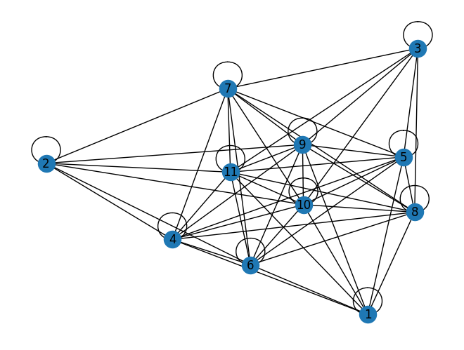
We can visualize the graph that defines this instance using the Q matrix as the adjacency matrix of a graph.
G = nx.from_numpy_array(Q)
nx.draw(G, with_labels=True, labels={i: i + 1 for i in G.nodes()})
plt.show()
Let’s define a QUBO model and then solve it using DWaves code for complete enumeration and simulated annealing (eventually with Quantum annealiing too!).
model = dimod.BinaryQuadraticModel.from_qubo(Q, offset=Beta)
print(model)
BinaryQuadraticModel({0: -46.0, 1: -44.0, 2: -44.0, 3: -92.0, 4: -92.0, 5: -92.0, 6: -91.0, 7: -92.0, 8: -139.0, 9: -138.0, 10: -139.0}, {(3, 0): 96.0, (3, 1): 96.0, (4, 0): 96.0, (4, 2): 96.0, (4, 3): 96.0, (5, 0): 96.0, (5, 1): 96.0, (5, 3): 192.0, (5, 4): 96.0, (6, 1): 96.0, (6, 2): 96.0, (6, 3): 96.0, (6, 4): 96.0, (6, 5): 96.0, (7, 0): 96.0, (7, 2): 96.0, (7, 3): 96.0, (7, 4): 192.0, (7, 5): 96.0, (7, 6): 96.0, (8, 0): 96.0, (8, 1): 96.0, (8, 2): 96.0, (8, 3): 192.0, (8, 4): 192.0, (8, 5): 192.0, (8, 6): 192.0, (8, 7): 192.0, (9, 0): 96.0, (9, 1): 96.0, (9, 2): 96.0, (9, 3): 192.0, (9, 4): 192.0, (9, 5): 192.0, (9, 6): 192.0, (9, 7): 192.0, (9, 8): 288.0, (10, 0): 96.0, (10, 1): 96.0, (10, 2): 96.0, (10, 3): 192.0, (10, 4): 192.0, (10, 5): 192.0, (10, 6): 192.0, (10, 7): 192.0, (10, 8): 288.0, (10, 9): 288.0}, 144.0, 'BINARY')
Since the problem is relatively small (11 variables, combinations), we can afford to enumerate all the solutions.
exactSampler = dimod.reference.samplers.ExactSolver()
exactSamples = exactSampler.sample(model)
# Some useful functions to get plots
def sample_label(sample):
return ''.join(str(int(sample[i])) for i in sorted(sample))
def format_solution(sample, vartype):
if vartype == dimod.BINARY:
return sample_label(sample)
return {i + 1: int(sample[i]) for i in sorted(sample)}
def best_samples(results):
ordered = list(results.data(['sample', 'energy'], sorted_by='energy'))
best_energy = ordered[0].energy
best = [datum.sample for datum in ordered if np.isclose(datum.energy, best_energy)]
return best, best_energy
def unique_formatted_solutions(samples, vartype):
unique = []
seen = set()
for sample in samples:
formatted = format_solution(sample, vartype)
key = formatted if isinstance(formatted, str) else tuple(formatted.items())
if key in seen:
continue
seen.add(key)
unique.append(formatted)
return unique
def plot_enumerate(results, title=None):
plt.figure()
ordered = list(results.data(['sample', 'energy'], sorted_by='energy'))
energies = [datum.energy for datum in ordered]
samples = np.arange(len(energies))
plt.bar(samples, energies)
tick_step = max(1, len(samples) // 12)
plt.xticks(samples[::tick_step])
plt.xlabel('solution index (sorted by energy)')
plt.ylabel('Energy')
plt.title(str(title))
plt.tight_layout()
plt.show()
def report_best_solutions(results, model_name):
best, best_energy = best_samples(results)
print(f'Best {model_name} objective value: {best_energy}')
print('Minimizing solution(s):', unique_formatted_solutions(best, results.vartype))
def plot_samples(results, title=None):
plt.figure()
if results.vartype == dimod.BINARY:
samples = [sample_label(datum.sample) for datum in results.data(['sample'], sorted_by=None)]
plt.xlabel('bitstring for solution')
else:
samples = np.arange(len(results))
plt.xlabel('solution')
counts = Counter(samples)
total = len(samples)
for key in counts:
counts[key] /= total
df = pd.DataFrame.from_dict(counts, orient='index').sort_index()
df.plot(kind='bar', legend=None)
plt.xticks(rotation=80)
plt.ylabel('Probabilities')
plt.title(str(title))
plt.tight_layout()
plt.show()
def plot_energies(results, title=None, skip=1):
energies = results.data_vectors['energy']
occurrences = results.data_vectors['num_occurrences']
counts = {}
total = sum(occurrences)
for index, energy in enumerate(energies):
counts[energy] = counts.get(energy, 0) + occurrences[index]
for key in counts:
counts[key] /= total
df = pd.DataFrame.from_dict(counts, orient='index').sort_index()
ax = df.plot(kind='bar', legend=None)
plt.xlabel('Energy')
plt.ylabel('Probabilities')
ax.set_xticklabels([tick if not i % skip else '' for i, tick in enumerate(ax.get_xticklabels())])
plt.title(str(title))
plt.tight_layout()
plt.show()
print('minimum energy:', min(energies))
plot_enumerate(exactSamples, title='Enumerate all solutions')
plot_energies(exactSamples, title='Enumerate all solutions', skip=10)
report_best_solutions(exactSamples, 'QUBO')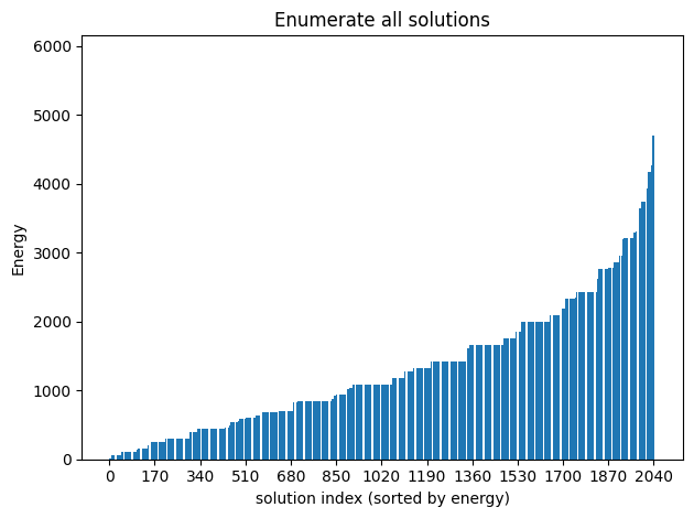
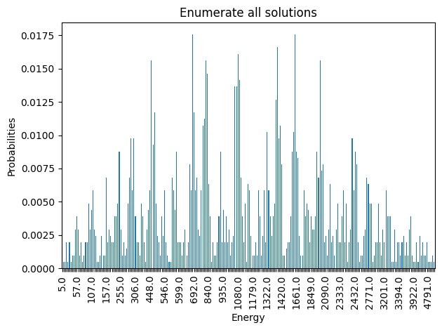
minimum energy: 5.0
Best QUBO objective value: 5.0
Minimizing solution(s): ['00000000001', '00000000100']
Let’s now solve this QUBO via traditional Integer Programming.
# We do not need to worry about the transformation to QUBO since dimod takes care of it.
Q, c = model.to_qubo()

# Define the model
model_pyo = pyo.ConcreteModel(name='QUBO example as an IP')

I = range(len(model))
J = range(len(model))
model_pyo.x = pyo.Var(I, domain=pyo.Binary)
model_pyo.y = pyo.Var(I, J, domain=pyo.Binary)

obj_expr = c

# Add model constraints
model_pyo.c1 = pyo.ConstraintList()
model_pyo.c2 = pyo.ConstraintList()
model_pyo.c3 = pyo.ConstraintList()
for (i, j) in Q.keys():
    if i != j:
        model_pyo.c1.add(model_pyo.y[i, j] >= model_pyo.x[i] + model_pyo.x[j] - 1)
        model_pyo.c2.add(model_pyo.y[i, j] <= model_pyo.x[i])
        model_pyo.c3.add(model_pyo.y[i, j] <= model_pyo.x[j])
        obj_expr += Q[i, j] * model_pyo.y[i, j]
    else:
        obj_expr += Q[i, j] * model_pyo.x[i]

model_pyo.objective = pyo.Objective(expr=obj_expr, sense=pyo.minimize)
print(f'Linearized QUBO IP with {len(I)} binary x variables and {len(I) * len(I)} auxiliary y variables.')
Linearized QUBO IP with 11 binary x variables and 121 auxiliary y variables.
We can solve the linearized QUBO reformulation with HiGHS, an open-source MILP solver that is available both in the repo-managed Python environment and through the Colab setup cell above.
# The Colab setup cell installs HiGHS when needed.
# Define the HiGHS solver
opt_highs = Highs()
# We could also use another MILP solver, e.g. Gurobi or CPLEX, through Pyomo.
# Solve the reformulated QUBO with HiGHS
result_obj = opt_highs.solve(model_pyo)
qubo_ip_active = [i + 1 for i in I if pyo.value(model_pyo.x[i]) > 0.5]
print(f'Objective value: {pyo.value(model_pyo.objective):.1f}')
print(f'Active binary variables (1-based): {qubo_ip_active}')
Objective value: 5.0
Active binary variables (1-based): [11]
We observe that both the exact enumeration and the HiGHS reformulation attain the minimum QUBO objective value of 5. In 1-based mathematical indexing, the two minimizing binary solutions have either or , with all other entries equal to 0.
Python displays the raw sampler dictionaries with 0-based keys, so these same two solutions appear at indices 8 and 10 in the direct enumeration output.
Ising model
This notebook will explain the basics of the Ising model. In order to implement the different Ising models we will use D-Wave’s packages dimod and neal, for defining the Ising model and solving it with simulated annealing, respectively. When posing the problems as integer programs, we will model using Pyomo, an open-source Python package that provides flexible access to different solvers and a general modeling framework for linear and nonlinear integer programs. The integer-programming reformulation below converts the Ising model to an equivalent QUBO and then solves the resulting MILP with the open-source HiGHS solver.
Problem statement
We pose the Ising problem as the following optimization problem:
where we optimize over spins , on a constrained graph , where the quadratic coefficients are and the linear coefficients are . We also include an arbitrary offset of the Ising model .
# These could also be simple lists and numpy matrices
h = {0: 145.0, 1: 122.0, 2: 122.0, 3: 266.0, 4: 266.0, 5: 266.0, 6: 242.5, 7: 266.0, 8: 386.5, 9: 387.0, 10: 386.5}
J = {(0, 3): 24.0, (0, 4): 24.0, (0, 5): 24.0, (0, 7): 24.0, (0, 8): 24.0, (0, 9): 24.0, (0, 10): 24.0, (1, 3): 24.0, (1, 5): 24.0, (1, 6): 24.0, (1, 8): 24.0, (1, 9): 24.0, (1, 10): 24.0, (2, 4): 24.0, (2, 6): 24.0, (2, 7): 24.0, (2, 8): 24.0, (2, 9): 24.0, (2, 10): 24.0, (3, 4): 24.0, (3, 5): 48.0, (3, 6): 24.0, (3, 7): 24.0, (3, 8): 48.0, (3, 9): 48.0, (3, 10): 48.0, (4, 5): 24.0, (4, 6): 24.0, (4, 7): 48.0, (4, 8): 48.0, (4, 9): 48.0, (4, 10): 48.0, (5, 6): 24.0, (5, 7): 24.0, (5, 8): 48.0, (5, 9): 48.0, (5, 10): 48.0, (6, 7): 24.0, (6, 8): 48.0, (6, 9): 48.0, (6, 10): 48.0, (7, 8): 48.0, (7, 9): 48.0, (7, 10): 48.0, (8, 9): 72.0, (8, 10): 72.0, (9, 10): 72.0}
cI = 1319.5

model_ising = dimod.BinaryQuadraticModel.from_ising(h, J, offset=cI)
Since the problem is relatively small (11 variables, combinations), we can afford to enumerate all the solutions.
exactSamples = exactSampler.sample(model_ising)plot_enumerate(exactSamples, title='Enumerate all solutions')
plot_energies(exactSamples, title='Enumerate all solutions')
report_best_solutions(exactSamples, 'Ising')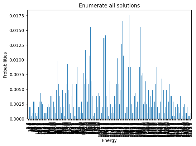
minimum energy: 5.0
Best Ising objective value: 5.0
Minimizing solution(s): [{1: -1, 2: -1, 3: -1, 4: -1, 5: -1, 6: -1, 7: -1, 8: -1, 9: 1, 10: -1, 11: -1}, {1: -1, 2: -1, 3: -1, 4: -1, 5: -1, 6: -1, 7: -1, 8: -1, 9: -1, 10: -1, 11: 1}]
Let’s now solve this Ising Model via traditional Integer Programming.
# We do not need to worry about the transformation from Ising to QUBO since dimod takes care of it.
Q, c = model_ising.to_qubo()

# Define the model
model_ising_pyo = pyo.ConcreteModel(name='Ising example as an IP')

I = range(len(h))
J = range(len(h))
model_ising_pyo.x = pyo.Var(I, domain=pyo.Binary)
model_ising_pyo.y = pyo.Var(I, J, domain=pyo.Binary)

obj_expr = c

# Add model constraints
model_ising_pyo.c1 = pyo.ConstraintList()
model_ising_pyo.c2 = pyo.ConstraintList()
model_ising_pyo.c3 = pyo.ConstraintList()
for (i, j) in Q.keys():
    if i != j:
        model_ising_pyo.c1.add(model_ising_pyo.y[i, j] >= model_ising_pyo.x[i] + model_ising_pyo.x[j] - 1)
        model_ising_pyo.c2.add(model_ising_pyo.y[i, j] <= model_ising_pyo.x[i])
        model_ising_pyo.c3.add(model_ising_pyo.y[i, j] <= model_ising_pyo.x[j])
        obj_expr += Q[i, j] * model_ising_pyo.y[i, j]
    else:
        obj_expr += Q[i, j] * model_ising_pyo.x[i]

model_ising_pyo.objective = pyo.Objective(expr=obj_expr, sense=pyo.minimize)
print(f'Binary reformulation of the Ising model with {len(I)} x variables and {len(I) * len(I)} auxiliary y variables.')
Binary reformulation of the Ising model with 11 x variables and 121 auxiliary y variables.
# Solve the reformulated Ising model with HiGHS
result_obj = opt_highs.solve(model_ising_pyo)
ising_ip_active = [i + 1 for i in I if pyo.value(model_ising_pyo.x[i]) > 0.5]
print(f'Objective value: {pyo.value(model_ising_pyo.objective):.1f}')
print(f'Active binary variables (1-based): {ising_ip_active}')
Objective value: 5.0
Active binary variables (1-based): [11]
Both the exact enumeration and the HiGHS reformulation attain the minimum Ising objective value of 5. In spin variables, the two minimizing states have either or , with all other spins equal to -1. After converting the Ising model to the binary QUBO form for the MILP solve, those same minima appear as or , with all other binary variables equal to 0.
Let’s go back to the slides
We can also solve this problem using Simulated Annealing
simAnnSampler = neal.SimulatedAnnealingSampler()
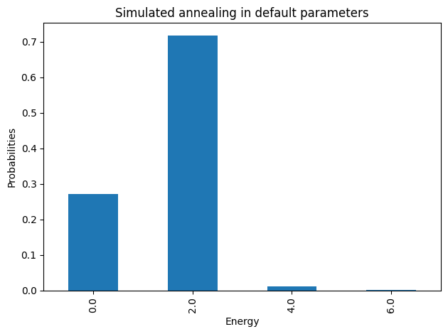
simAnnSamples = simAnnSampler.sample(model_ising, num_reads=1000)plot_enumerate(simAnnSamples, title='Simulated annealing in default parameters')
plot_energies(simAnnSamples, title='Simulated annealing in default parameters')
report_best_solutions(simAnnSamples, 'Ising')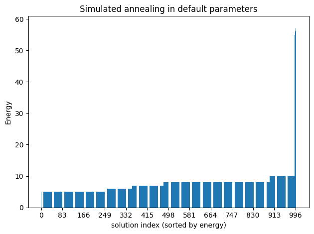
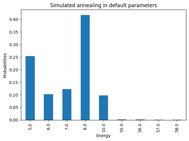
minimum energy: 5.0
Best Ising objective value: 5.0
Minimizing solution(s): [{1: -1, 2: -1, 3: -1, 4: -1, 5: -1, 6: -1, 7: -1, 8: -1, 9: 1, 10: -1, 11: -1}, {1: -1, 2: -1, 3: -1, 4: -1, 5: -1, 6: -1, 7: -1, 8: -1, 9: -1, 10: -1, 11: 1}]
simAnnSamples.info{'beta_range': [np.float64(0.00041111932417553103),
np.float64(0.1458971970580513)],
'beta_schedule_type': 'geometric',
'timing': {'preprocessing_ns': 1797248,
'sampling_ns': 164514819,
'postprocessing_ns': 329020}}Let’s go back to the slides
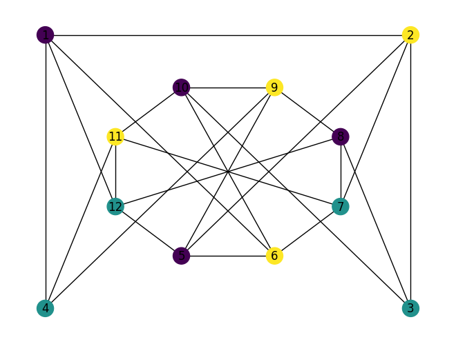
Let’s solve the graph coloring problem in the slides using QUBO.
Vertex -coloring of graphs
Given a graph , where is the set of vertices and is the set of edges of , and a positive integer , we ask if it is possible to assign a color to every vertex from , such that adjacent vertices have different colors assigned.
has 12 vertices and 23 edges. We ask if the graph is 3–colorable. Let’s first encode and using Julia’s built–in data structures:
Note: This tutorial is heavily inspired by D-Wave’s Map coloring of Canada example found here.
import dwavebinarycsp
/tmp/ipykernel_1152980/4003106872.py:1: DeprecationWarning: dwavebinarycsp is deprecated and will be removed in Ocean 10. For solving problems with constraints, we recommend using the hybrid solvers in the Leap service. You can find documentation for the hybrid solvers at https://docs.ocean.dwavesys.com.
  import dwavebinarycsp
V = range(1, 12+1)
E = [(1,2),(2,3),(1,4),(1,6),(1,12),(2,5),(2,7),(3,8),(3,10),(4,11),(4,9),(5,6),(6,7),(7,8),(8,9),(9,10),(10,11),(11,12),(5,12),(5,9),(6,10),(7,11),(8,12)]
layout = {i: [np.cos((2*i+1)*np.pi/8),np.sin((2*i+1)*np.pi/8)] for i in np.arange(5,13)}
layout[1] = [-1.5,1.5]
layout[2] = [1.5,1.5]
layout[3] = [1.5,-1.5]
layout[4] = [-1.5,-1.5]
G = nx.Graph()
G.add_edges_from(E)
nx.draw(G, with_labels=True, pos=layout)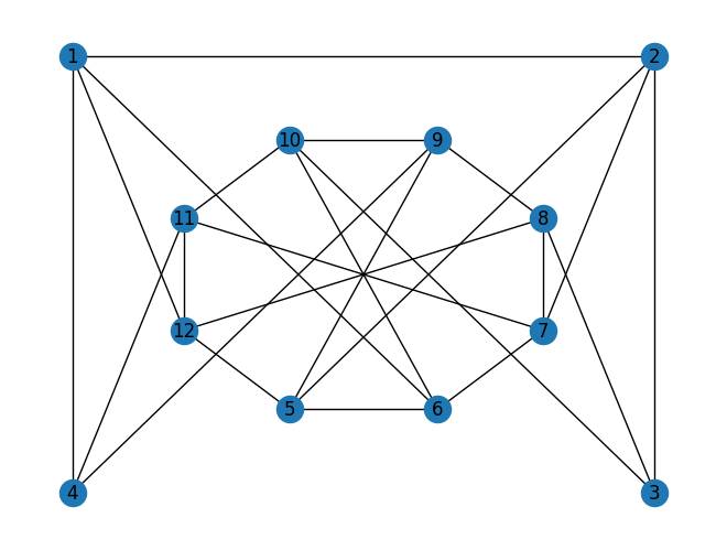
# Function for the constraint that two nodes with a shared edge not both select
# one color
def not_both_1(v, u):
    return not (v and u)

# Valid configurations for the constraint that each node select a single color, in this case we want to use 3 colors
one_color_configurations = {(0, 0, 1), (0, 1, 0), (1, 0, 0)}
colors = len(one_color_configurations)

# Create a binary constraint satisfaction problem
csp = dwavebinarycsp.ConstraintSatisfactionProblem(dwavebinarycsp.BINARY)

# Add constraint that each node select a single color
for node in V:
    variables = ['x'+str(node)+','+str(i) for i in range(colors)]
    csp.add_constraint(one_color_configurations, variables)

# Add constraint that each pair of nodes with a shared edge not both select one color
for edge in E:
    v, u = edge
    for i in range(colors):
        variables = ['x'+str(v)+','+str(i), 'x'+str(u)+','+str(i)]
        csp.add_constraint(not_both_1, variables)
Defining the Binary Quadratic Model (QUBO) using the CSP library we have:
bqm = dwavebinarycsp.stitch(csp)
simAnnSamples = simAnnSampler.sample(bqm, num_reads=1000)
plot_enumerate(simAnnSamples, title='Simulated annealing in default parameters')
plot_energies(simAnnSamples, title='Simulated annealing in default parameters')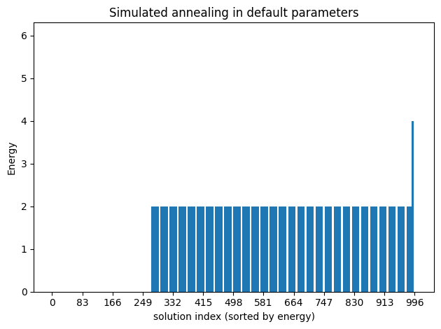
minimum energy: 0.0
Because of precision issues in the translation to a BQM, we may obtain very tiny coefficients that should be zero. In any case, since this is a constraint satisfaction problem, any of the solutions with energy ~0 is a valid coloring.
# Check that a good solution was found
sample = simAnnSamples.first.sample     # doctest: +SKIP
if not csp.check(sample):           # doctest: +SKIP
        print("Failed to color map. Try sampling again.")
else:
        print(sample)
{'x1,0': np.int8(1), 'x1,1': np.int8(0), 'x1,2': np.int8(0), 'x10,0': np.int8(1), 'x10,1': np.int8(0), 'x10,2': np.int8(0), 'x11,0': np.int8(0), 'x11,1': np.int8(0), 'x11,2': np.int8(1), 'x12,0': np.int8(0), 'x12,1': np.int8(1), 'x12,2': np.int8(0), 'x2,0': np.int8(0), 'x2,1': np.int8(0), 'x2,2': np.int8(1), 'x3,0': np.int8(0), 'x3,1': np.int8(1), 'x3,2': np.int8(0), 'x4,0': np.int8(0), 'x4,1': np.int8(1), 'x4,2': np.int8(0), 'x5,0': np.int8(1), 'x5,1': np.int8(0), 'x5,2': np.int8(0), 'x6,0': np.int8(0), 'x6,1': np.int8(0), 'x6,2': np.int8(1), 'x7,0': np.int8(0), 'x7,1': np.int8(1), 'x7,2': np.int8(0), 'x8,0': np.int8(1), 'x8,1': np.int8(0), 'x8,2': np.int8(0), 'x9,0': np.int8(0), 'x9,1': np.int8(0), 'x9,2': np.int8(1)}
# Function that plots a returned sample
def plot_map(sample):
    # Translate from binary to integer color representation
    color_map = {}
    for node in V:
          for i in range(colors):
            if sample['x'+str(node)+','+str(i)]:
                color_map[node] = i
    # Plot the sample with color-coded nodes
    node_colors = [color_map.get(node) for node in G.nodes()]
    nx.draw(G, with_labels=True, pos=layout, node_color=node_colors)
    plt.show()
plot_map(sample)