Introduction to Mathematical Programming
David E. Bernal NeiraDavidson School of Chemical Engineering, Purdue University
Pedro Maciel Xavier
Davidson School of Chemical Engineering, Purdue University
Azain Khalid
Department of Computer Science, Purdue University
Undergraduate Researcher


Environment setup
For local execution from the repository root, run make setup-julia NOTEBOOK=notebooks_jl/1-MathProg.ipynb before launching Jupyter. This notebook now uses its own Julia project under notebooks_jl/envs/1-MathProg/, so it does not install the QUBO and D-Wave stack.
This notebook should open directly with the Julia runtime in Google Colab. If it does not, switch the runtime before running the next cell.
The setup cell will clone SECQUOIA/QuIP into the Colab workspace when needed, activate notebooks_jl/envs/1-MathProg/Project.toml, instantiate only the Julia packages used in this notebook, and print progress for clone, activate, instantiate, and package-load steps. Package precompilation still happens as needed during setup. The first Colab run can still take several minutes.
function load_notebook_bootstrap()
    candidates = (
        joinpath(pwd(), "scripts", "notebook_bootstrap.jl"),
        joinpath(pwd(), "..", "scripts", "notebook_bootstrap.jl"),
        joinpath(pwd(), "QuIP", "scripts", "notebook_bootstrap.jl"),
        joinpath("/content", "QuIP", "scripts", "notebook_bootstrap.jl"),
    )

    for candidate in candidates
        if isfile(candidate)
            include(candidate)
            return nothing
        end
    end

    in_colab = haskey(ENV, "COLAB_RELEASE_TAG") || haskey(ENV, "COLAB_JUPYTER_IP") || isdir(joinpath("/content", "sample_data"))
    if in_colab
        repo_dir = get(ENV, "QUIP_REPO_DIR", joinpath(pwd(), "QuIP"))
        if !isdir(repo_dir)
            println("[bootstrap] Cloning SECQUOIA/QuIP into $repo_dir")
            run(`git clone --depth 1 https://github.com/SECQUOIA/QuIP.git $repo_dir`)
        end
        include(joinpath(repo_dir, "scripts", "notebook_bootstrap.jl"))
        return nothing
    end

    error("Could not locate scripts/notebook_bootstrap.jl from $(pwd()).")
end

load_notebook_bootstrap()

BOOTSTRAP = QuIPNotebookBootstrap.bootstrap_notebook("1-MathProg")

QUIP_REPO_DIR = BOOTSTRAP.repo_dir
JULIA_NOTEBOOKS_DIR = BOOTSTRAP.notebooks_dir
JULIA_PROJECT_DIR = BOOTSTRAP.project_dir
IN_COLAB = BOOTSTRAP.in_colab
Mathematical Programming (Julia)
Modeling
The solution to optimization problems requires the development of a mathematical model. Here we will model an example given in the lecture and see how an integer program can be solved practically. This example will use as modeling language JuMP. This open-source Julia package provides flexible access to different solvers and a general modeling framework for linear and nonlinear integer programs. The examples solved here will make use of open-source solvers GLPK and HiGHS for linear and mixed-integer linear programming, IPOPT for interior-point (non)linear programming, BONMIN for convex integer nonlinear programming, and COUENNE together with SCIP for nonconvex integer nonlinear programming.
Problem statement
Suppose there is a company that produces two different products, A and B, which can be sold at different values, and per unit, respectively. The company only counts with a single machine with electricity usage of at most 17kW/day. Producing each A and B consumes and , respectively. Besides, the company can only produce at most 2 more units of B than A per day.
Linear Programming
This is a valid model, but it would be easier to solve if we had a mathematical representation. Assuming the units produced of A are and of B are we have
if !@isdefined(Plots)
    using Plots
end
function plot_lp(;ns::Integer = 1_000, sol = nothing)
    # Create empty plot
    plt = plot(;
        plot_title="LP Feasible Region",
        plot_titlevspan=0.1,
    )

    # Generate the feasible region plot of this problem
    x1 = x2 = range(-0.5, 3.5; length = ns)

    # Objective: max 5.5x₁ + 2.1x₂
    z(x1, x2) = 5.5x1 + 2.1x2

    # Constraints
    isfeasible(x1, x2) = (x1 >= 0)      && # Bound: x1 ≥ 0
                         (x2 >= 0)      && # Bound: x2 ≥ 0
                         (x2 <= x1 + 2) && # Constraint 1: x₂ ≤ x₁ + 2
                         (8x1 + 2x2 <= 17) # Constraint 2: 8 x₁ + 2 x₂ ≤ 17

    # Heatmap function
    f(x1, x2) = ifelse(isfeasible(x1, x2), z(x1, x2), NaN)

    # Plot feasible region
    heatmap!(
        plt, x1, x2, f;
        legend=:topright,
        title=raw"$ \max ~ z = 5.5 x_1 + 2.1 x_2 $",
        xlims=extrema(x1),
        ylims=extrema(x2),
        xlabel=raw"$ x_1 $",
        ylabel=raw"$ x_2 $",
    )

    # Make plots of constraints
    plot!(plt, x1, (x1) -> x1 + 2;
        label=raw"$ x_2 \leq x_1 + 2 $",
        color=:green,
    )
    plot!(plt, x1, (x1) -> (17 - 8x1) / 2;
        label=raw"$ 8 x_1 + 2 x_2 \leq 17 $",
        color=:blue,
    )

    # Nonnegativitivy constraints
    plot!(plt, zeros(ns), x2;
        label=raw"$ x_1 \geq 0 $",
        color=:purple,
    )
    plot!(plt, x1, zeros(ns);
        label=raw"$ x_2 \geq 0 $",
        color=:red,
    )

    if sol !== nothing
        # Optimal solution
        scatter!(plt, [sol[1]], [sol[2]];
            label=raw"$ (x_1^\ast, x_2^\ast) $",
            marker_z=z,
            markershape=:star8,
        )
    end

    return plt
end

plot_lp()if !@isdefined(JuMP)
using JuMP
end
# Define empty model
lp_model = Model()

# Define the variables
@variable(lp_model, x[1:2] >= 0)

# Define the objective function
@objective(lp_model, Max, 5.5x[1] + 2.1x[2])

# Define the constraints
@constraint(lp_model, c1, x[2] <= x[1] + 2)

@constraint(lp_model, c2, 8x[1] + 2x[2] <= 17)

# Print the model
print(lp_model)if !@isdefined(GLPK)
using GLPK
end
# Here we solve the optimization problem with GLPK
set_optimizer(lp_model, GLPK.Optimizer)

set_silent(lp_model)

optimize!(lp_model)

# Retrieve solution value for "x"
lp_x = value.(x)

# Display solution of the problem
println(solution_summary(lp_model))
println("* x = $lp_x")
We observe that the optimal solution of this problem is , leading to a profit of 14.08.
if !@isdefined(HiGHS)
    using HiGHS
end
# With HiGHS instead:
set_optimizer(lp_model, HiGHS.Optimizer)

set_silent(lp_model)

optimize!(lp_model)

# Retrieve solution value for "x"
lp_x = value.(x)

# Display solution of the problem
println(solution_summary(lp_model))
println("* x = $lp_x")
plot_lp(;sol = lp_x)HiGHS recovers the same LP optimum as GLPK. GLPK and HiGHS are open-source LP/MIP solvers, and HiGHS is a good default for this notebook. We can also solve the LP relaxation with the interior-point solver IPOPT, which extends naturally to nonlinear programs. In mixed-integer models, however, IPOPT alone is not enough because it does not enforce integrality.
if !@isdefined(Ipopt)
    using Ipopt
end
# Using Ipopt for an interior point method
set_optimizer(lp_model, Ipopt.Optimizer)
set_silent(lp_model)

optimize!(lp_model)

# Retrieve solution value for "x"
lp_x = value.(x)

# Display solution of the problem
println(solution_summary(lp_model))
println("* x = $lp_x")
We obtain the same result as previously, but notice that the interior point method reports a solution subject to a certain tolerance, given by its convergence properties when it can get infinitesimally close (but not directly at) the boundary of the feasible region.
The LP model is a useful baseline because it solves quickly, and it gives us a reference objective before we add nonlinear structure or impose integrality. It is also an upper bound on the later integer model.
Nonlinear Programming
Before imposing integrality, we can add a convex nonlinear constraint while keeping the variables continuous. This gives the following nonlinear program (NLP):
function plot_nlp(; ns::Integer = 1_000, sol = nothing)
    plt = plot(;
        plot_title="NLP Feasible Region",
        plot_titlevspan=0.1,
    )

    x1 = x2 = range(-0.5, 3.5; length = ns)

    z(x1, x2) = 5.5x1 + 2.1x2

    isfeasible(x1, x2) = (x1 >= 0)           &&
                         (x2 >= 0)           &&
                         (x2 <= x1 + 2)      &&
                         (8x1 + 2x2 <= 17)   &&
                         ((x2 - 1)^2 <= 2 - x1)

    f(x1, x2) = ifelse(isfeasible(x1, x2), z(x1, x2), NaN)
    g(x1, x2) = ifelse(isfeasible(x1, x2), 1.0, NaN)

    heatmap!(
        plt, x1, x2, f;
        legend=:topright,
        title=raw"$ z = 5.5 x_1 + 2.1 x_2 $",
        xlims=extrema(x1),
        ylims=extrema(x2),
        xlabel=raw"$ x_1 $",
        ylabel=raw"$ x_2 $",
    )

    heatmap!(
        plt, x1, x2, g;
        alpha=0.4,
        color=:white,
        colorbar_entry=false,
        xlims=extrema(x1),
        ylims=extrema(x2),
    )

    plot!(plt, x1, (x1) -> x1 + 2;
        label=raw"$ x_2 \leq x_1 + 2 $",
        color=:green,
    )
    plot!(plt, x1, (x1) -> (17 - 8x1) / 2;
        label=raw"$ 8 x_1 + 2 x_2 \leq 17 $",
        color=:blue,
    )
    plot!(plt, 2 .- (x1 .- 1) .^ 2, x1;
        label=raw"$ (x_2 - 1)^2 \leq 2 - x_1 $",
        color=:orange,
    )
    plot!(plt, zeros(ns), x2;
        label=raw"$ x_1 \geq 0 $",
        color=:purple,
    )
    plot!(plt, x1, zeros(ns);
        label=raw"$ x_2 \geq 0 $",
        color=:red,
    )

    if sol !== nothing
        scatter!(plt, [sol[1]], [sol[2]];
            label=raw"$ (x_1^\ast, x_2^\ast) $",
            marker_z=z,
            markershape=:star8,
        )
    end

    return plt
end

plot_nlp()
# Define and solve the nonlinear program
nlp_model = copy(lp_model)
x = nlp_model[:x]
@constraint(nlp_model, c3, (x[2] - 1)^2 <= 2 - x[1])
print(nlp_model)

set_optimizer(nlp_model, Ipopt.Optimizer)
set_silent(nlp_model)

optimize!(nlp_model)

nlp_x = value.(x)

println(solution_summary(nlp_model))
println("* x = $nlp_x")
plot_nlp(; sol = nlp_x)
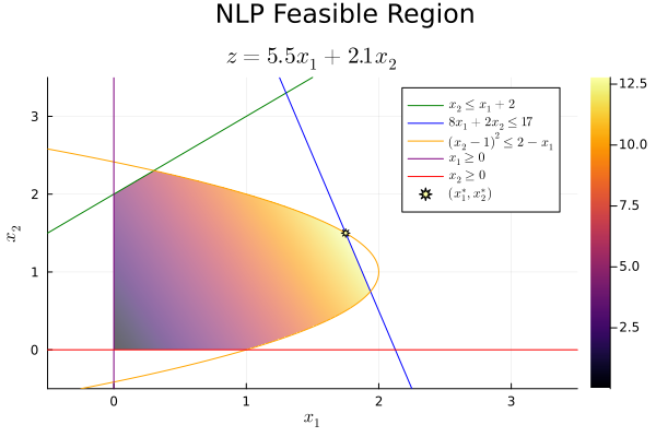
Here the continuous NLP solution is approximately with objective 12.775. Compared with the LP solution, the convex nonlinear constraint bends the feasible region and lowers the optimum, but the problem is still continuous because no integrality has been imposed yet.
Integer Programming
Now let’s consider that only integer units of each product can be produced, namely
function plot_ilp(;ns::Integer = 1_000, sol = nothing)
    # Create empty plot
    plt = plot(;
        plot_title="ILP Feasible Region",
        plot_titlevspan=0.1,
    )

    # Generate the feasible region plot of this problem
    x1 = x2 = range(-0.5, 3.5; length = ns)

    # Objective: max 5.5x₁ + 2.1x₂
    z(x1, x2) = 5.5x1 + 2.1x2

    # Constraints
    isfeasible(x1, x2) = (x1 >= 0)      && # Bound: x1 ≥ 0
                         (x2 >= 0)      && # Bound: x2 ≥ 0
                         (x2 <= x1 + 2) && # Constraint 1: x₂ ≤ x₁ + 2
                         (8x1 + 2x2 <= 17) # Constraint 2: 8 x₁ + 2 x₂ ≤ 17

    # Optimal Solution
    isoptimal(x1, x2) = (sol !== nothing) && (x1 ≈ sol[1] && x2 ≈ sol[2])

    # Heatmap functions
    f(x1, x2) = ifelse(isfeasible(x1, x2), z(x1, x2), NaN)
    g(x1, x2) = ifelse(isfeasible(x1, x2), 1.0, NaN)

    # Plot relaxed feasible region
    heatmap!(
        plt, x1, x2, f;
        legend=:topright,
        title=raw"$ z = 5.5 x_1 + 2.1 x_2 $",
        xlims=extrema(x1),
        ylims=extrema(x2),
        xlabel=raw"$ x_1 $",
        ylabel=raw"$ x_2 $",
    )

    # Dim relaxed feasible region
    heatmap!(
        plt, x1, x2, g;
        alpha=0.4,
        color=:white,
        colorbar_entry=false,
        xlims=extrema(x1),
        ylims=extrema(x2),
    )

    # Make plots of constraints
    plot!(plt, x1, (x1) -> x1 + 2;
        label=raw"$ x_2 \leq x_1 + 2 $",
        color=:green,
    )
    plot!(plt, x1, (x1) -> (17 - 8x1) / 2;
        label=raw"$ 8 x_1 + 2 x_2 \leq 17 $",
        color=:blue,
    )

    # Nonnegativitivy constraints
    plot!(plt, zeros(ns), x2;
        label=raw"$ x_1 \geq 0 $",
        color=:purple,
    )
    plot!(plt, x1, zeros(ns);
        label=raw"$ x_2 \geq 0 $",
        color=:red,
    )

    # Feasible solutions
    xi = []
    xj = []

    for i = 0:4, j = 0:4
        if isfeasible(i, j) && !isoptimal(i, j)
            push!(xi, i)
            push!(xj, j)
        end
    end

    scatter!(plt, xi, xj;
        label=raw"$ (x_1, x_2) \in \mathbb{Z}^2 $",
        marker_z=z,
    )

    if sol !== nothing
        # Optimal solution
        scatter!(plt, [sol[1]], [sol[2]];
            label=raw"$ (x_1^\ast, x_2^\ast) $",
            marker_z=z,
            markershape=:star8,
        )
    end

    return plt
end

plot_ilp()# Copy model
ilp_model = copy(lp_model)
# Retrieve variable reference
x = ilp_model[:x]
# Add integrality contraint: x₁, x₂ ∈ ℤ
set_integer.(x)
# Print the model
print(ilp_model)set_optimizer(ilp_model, HiGHS.Optimizer)
set_silent(ilp_model)
optimize!(ilp_model)
# Retrieve the optimal integer solution
ilp_x = value.(x)
println(solution_summary(ilp_model))
println("* x = $ilp_x")
Here the solution becomes with an objective of 11.8. Compared with the LP relaxation, the integer restriction shrinks the feasible set, so the best achievable profit is lower.
plot_ilp(; sol = ilp_x)Enumeration
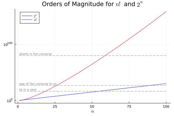
Enumerating all the possible solutions in this problem might be very efficient (there are only 8 feasible solutions), but we only know that from the plot. Assuming that we had upper bounds of 4 for both variables, the possible solutions would already rise to 16. With a larger number of variables, enumeration quickly becomes impractical. For binary variables (we can always “binarize” the integer variables), the number of possible solutions is .
In many other applications, the possible solutions come from permutations of the integer variables (e.g., assignment problems), which grow as with the size of the input.
This growth makes the problem get out of control fairly quickly.
if !@isdefined(SpecialFunctions)
    using SpecialFunctions
end
function plot_growth(n::Integer = 100)
    i = 1:n

    plt = plot(;
        title=raw"Orders of Magnitude for $ n! $ and $ 2^n $",
        xlabel=raw"$ n $",
        legend=:topleft,
        yscale=:log10,
    )

    plot!(plt, i, (i) -> 2.0^i; label=raw"$ 2^n $", color=:blue)
    plot!(plt, i, (i) -> SpecialFunctions.gamma(i + 1); label=raw"$ n! $", color=:red)

    plot!(plt, i, (i) -> 3.154E16; color=:gray, label = nothing, linestyle = :dash)
    annotate!(plt, first(i), 3.154E16, text("ns in a year", :gray, :left, :bottom, 7))

    plot!(plt, i, (i) -> 4.3E26; color=:gray, label = nothing, linestyle = :dash)
    annotate!(plt, first(i), 4.3E26, text("age of the universe in ns", :gray, :left, :bottom, 7))

    plot!(plt, i, (i) -> 6E79; color=:gray, label = nothing, linestyle = :dash)
    annotate!(plt, first(i), 6E79, text("atoms in the universe", :gray, :left, :bottom, 7))

    return plt
end

plot_growth()
Integer convex nonlinear programming
If we keep the same convex nonlinear constraint and now require integer decisions, we obtain the following convex integer nonlinear program.
function plot_icnlp(; ns::Integer = 1_000, sol = nothing)
    # Create empty plot
    plt = plot(;
        plot_title="ICNLP Feasible Region",
        plot_titlevspan=0.1,
    )

    # Generate the feasible region plot of this problem
    x1 = x2 = range(-0.5, 3.5; length = ns)

    # Objective: max 5.5x₁ + 2.1x₂
    z(x1, x2) = 5.5x1 + 2.1x2

    # Constraints
    isfeasible(x1, x2) = (x1 >= 0)           && # Bound: x1 ≥ 0
                         (x2 >= 0)           && # Bound: x2 ≥ 0
                         (x2 <= x1 + 2)      && # Constraint 1: x₂ ≤ x₁ + 2
                         (8x1 + 2x2 <= 17)   && # Constraint 2: 8 x₁ + 2 x₂ ≤ 17
                         ((x2 - 1)^2 <= 2 - x1) # Constraint 3: (x₂ - 1)² ≤ 2 - x₁

    # Optimal Solution
    isoptimal(x1, x2) = (sol !== nothing) && (x1 ≈ sol[1] && x2 ≈ sol[2])

    # Heatmap functions
    f(x1, x2) = ifelse(isfeasible(x1, x2), z(x1, x2), NaN)
    g(x1, x2) = ifelse(isfeasible(x1, x2), 1.0, NaN)

    # Plot relaxed feasible region
    heatmap!(
        plt, x1, x2, f;
        legend=:topright,
        title=raw"$ z = 5.5 x_1 + 2.1 x_2 $",
        xlims=extrema(x1),
        ylims=extrema(x2),
        xlabel=raw"$ x_1 $",
        ylabel=raw"$ x_2 $",
    )

    # Dim relaxed feasible region
    heatmap!(
        plt, x1, x2, g;
        alpha=0.4,
        color=:white,
        colorbar_entry=false,
        xlims=extrema(x1),
        ylims=extrema(x2),
    )

    # Make plots of constraints
    plot!(plt, x1, (x1) -> x1 + 2;
        label=raw"$ x_2 \leq x_1 + 2 $",
        color=:green,
    )
    plot!(plt, x1, (x1) -> (17 - 8x1) / 2;
        label=raw"$ 8 x_1 + 2 x_2 \leq 17 $",
        color=:blue,
    )
    plot!(plt, 2 .- (x1 .- 1) .^ 2, x1,;
        label=raw"$ (x_2 - 1)^2 \leq 2 - x_1 $",
        color=:orange,
    )

    # Nonnegativitivy constraints
    plot!(plt, zeros(ns), x2;
        label=raw"$ x_1 \geq 0 $",
        color=:purple,
    )
    plot!(plt, x1, zeros(ns);
        label=raw"$ x_2 \geq 0 $",
        color=:red,
    )

    # Feasible solutions
    xi = []
    xj = []

    for i = 0:4, j = 0:4
        if isfeasible(i, j) && !isoptimal(i, j)
            push!(xi, i)
            push!(xj, j)
        end
    end

    scatter!(plt, xi, xj;
        label=raw"$ (x_1, x_2) \in \mathbb{Z}^2 $",
        marker_z=z,
    )

    if sol !== nothing
        # Optimal solution
        scatter!(plt, [sol[1]], [sol[2]];
            label=raw"$ (x_1^\ast, x_2^\ast) $",
            marker_z=z,
            markershape=:star8,
        )
    end

    return plt
end

plot_icnlp()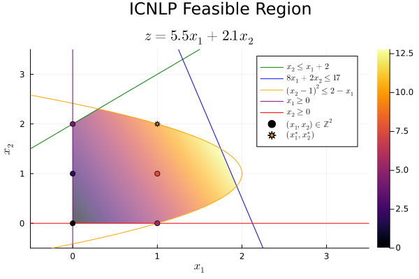
# Define the model
icnlp_model = copy(ilp_model)

# Retrieve variable reference
x = icnlp_model[:x]

# (x₂ - 1)² ≤ 2 - x₁
@constraint(icnlp_model, c3, (x[2] - 1)^2 <= 2 - x[1])

# Print the model
print(icnlp_model)# BONMIN solver
using AmplNLWriter
using Bonmin_jll
Bonmin_Optimizer() = AmplNLWriter.Optimizer(Bonmin_jll.amplexe);
set_optimizer(icnlp_model, Bonmin_Optimizer)

optimize!(icnlp_model)

icnlp_x = value.(x)

println(solution_summary(icnlp_model))
println("* x = $icnlp_x")
In this case the optimal solution becomes with an objective of 9.7. Compared with the continuous NLP, the same nonlinear geometry is still present, but the integer restriction removes the fractional optimum and lowers the best achievable profit again.
plot_icnlp(; sol = icnlp_x)Integer non-convex programming
The last constraint “the production of B minus 1 squared can only be greater than the production of A plus one half” can be incorporated in the following non-convex integer nonlinear program
function plot_incnlp(; ns::Integer = 1_000, sol = nothing)
    # Create empty plot
    plt = plot(;
        plot_title="Nonconvex INLP Feasible Region",
        plot_titlevspan=0.1,
    )

    # Generate the feasible region plot of this problem
    x1 = x2 = range(-0.5, 3.5; length = ns)

    # Objective: max 5.5x₁ + 2.1x₂
    z(x1, x2) = 5.5x1 + 2.1x2

    # Constraints
    isfeasible(x1, x2) = (x1 >= 0)              && # Bound: x1 ≥ 0
                         (x2 >= 0)              && # Bound: x2 ≥ 0
                         (x2 <= x1 + 2)         && # Constraint 1: x₂ ≤ x₁ + 2
                         (8x1 + 2x2 <= 17)      && # Constraint 2: 8 x₁ + 2 x₂ ≤ 17
                         ((x2 - 1)^2 <= 2 - x1) && # Constraint 3: (x₂ - 1)² ≤ 2 - x₁
                         ((x2 - 1)^2 >= 1/2 + x1)  # Constraint 4: (x₂ - 1)² ≥ 1/2 + x₁

    # Optimal Solution
    isoptimal(x1, x2) = (sol !== nothing) && (x1 ≈ sol[1] && x2 ≈ sol[2])

    # Heatmap functions
    f(x1, x2) = ifelse(isfeasible(x1, x2), z(x1, x2), NaN)
    g(x1, x2) = ifelse(isfeasible(x1, x2), 1.0, NaN)

    # Plot relaxed feasible region
    heatmap!(
        plt, x1, x2, f;
        legend=:topright,
        title=raw"$ \max ~ z = 5.5 x_1 + 2.1 x_2 $",
        xlims=extrema(x1),
        ylims=extrema(x2),
        xlabel=raw"$ x_1 $",
        ylabel=raw"$ x_2 $",
    )

    # Dim relaxed feasible region
    heatmap!(
        plt, x1, x2, g;
        alpha=0.4,
        color=:white,
        colorbar_entry=false,
        xlims=extrema(x1),
        ylims=extrema(x2),
    )

    # Make plots of constraints
    plot!(plt, x1, (x1) -> x1 + 2;
        label=raw"$ x_2 \leq x_1 + 2 $",
        color=:green,
    )
    plot!(plt, x1, (x1) -> (17 - 8x1) / 2;
        label=raw"$ 8 x_1 + 2 x_2 \leq 17 $",
        color=:blue,
    )
    plot!(plt, 2 .- (x1 .- 1) .^ 2, x1,;
        label=raw"$ (x_2 - 1)^2 \leq 2 - x_1 $",
        color=:orange,
    )
    plot!(plt, -1/2 .+ (x1 .- 1) .^ 2, x1,;
        label=raw"$ (x_2 - 1)^2 \geq \frac{1}{2} + x_1 $",
        color=:magenta,
    )

    # Nonnegativitivy constraints
    plot!(plt, zeros(ns), x2;
        label=raw"$ x_1 \geq 0 $",
        color=:purple,
    )
    plot!(plt, x1, zeros(ns);
        label=raw"$ x_2 \geq 0 $",
        color=:red,
    )

    # Feasible solutions
    xi = []
    xj = []

    for i = 0:4, j = 0:4
        if isfeasible(i, j) && !isoptimal(i, j)
            push!(xi, i)
            push!(xj, j)
        end
    end

    scatter!(plt, xi, xj;
        label=raw"$ (x_1, x_2) \in \mathbb{Z}^2 $",
        marker_z=z,
    )

    if sol !== nothing
        # Optimal solution
        scatter!(plt, [round(sol[1])], [round(sol[2])];
            label=raw"$ (x_1^\ast, x_2^\ast) $",
            marker_z=z,
            markershape=:star8,
        )
    end

    return plt
end

plot_incnlp()
# Define the model
incnlp_model = copy(icnlp_model)
# Retrieve variable reference
x = incnlp_model[:x]
# (x₂ - 1)² ≥ 1/2 + x₁
@constraint(incnlp_model, c4, (x[2] - 1)^2 >= 1/2 + x[1])
# Print the model
print(incnlp_model)# Trying to solve the problem with BONMIN we might obtain a good solution,
# but we have no global guarantees
set_optimizer(incnlp_model, Bonmin_Optimizer)
optimize!(incnlp_model)
if result_count(incnlp_model) > 0
incnlp_x = value.(x)
println("* x = $incnlp_x")
end
# Global MINLP solvers
using Couenne_jll
using SCIP

Couenne_Optimizer() = AmplNLWriter.Optimizer(Couenne_jll.amplexe);
# Solve the global MINLP with COUENNE
set_optimizer(incnlp_model, Couenne_Optimizer)

optimize!(incnlp_model)

println(solution_summary(incnlp_model))

if result_count(incnlp_model) > 0
    incnlp_x = value.(x)

    println("* x = $incnlp_x")
end
# Solve the same global MINLP directly with SCIP
scip_model = copy(incnlp_model)
x_scip = scip_model[:x]

set_optimizer(scip_model, SCIP.Optimizer)
set_silent(scip_model)

optimize!(scip_model)

println(solution_summary(scip_model))

if result_count(scip_model) > 0
    incnlp_scip_x = value.(x_scip)

    println("* x = $incnlp_scip_x")
end
COUENNE and SCIP both recover the global optimum , with objective 4.2. BONMIN may also find this point, but it does not provide a global certificate in this non-convex setting. This is the first section where solver guarantees become central: a local answer is not enough.
plot_incnlp(; sol = incnlp_x)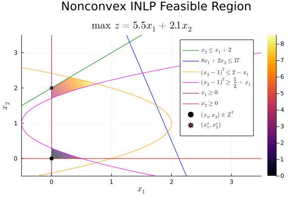
We are able to solve non-convex MINLP problems. However, the complexity of these problems leads to significant computational challenges that need to be tackled.
References
Commercial solver installation
Gurobi
Gurobi offers free academic licenses for students, faculty, and staff at recognized degree-granting institutions, and the current academic options include named-user, WLS, and site-license workflows. Because license types and setup steps change over time, use the current official pages for both eligibility and installation details:
Academic licenses: https://
www .gurobi .com /features /academic -cloud -license/ License setup: https://
support .gurobi .com /hc /en -us /articles /12872879801105 -How -do -I -retrieve -and -set -up -a -Gurobi -license
BARON
BARON remains a leading global MINLP solver, but its academic licensing is more restrictive: most academic users use discounted academic pricing, while free licenses are limited to specific partner-university programs listed on the vendor site. Since these terms can change, check the current license and FAQ pages before planning coursework around BARON: